Translate This Page

Logistic map approach to Gibbs excess free energies of a mixture
Pier Francesco Sciuto
DOWNLOAD PDF VERSION 
WARNING - PRESENT PAPER WAS REGISTERED IN 2006
Key words:
Logistic map, Verhulst, geochemistry, mistures
Abstract
Logistic maps can be a useful tool to describe Gibbs excess energy in multicomponent systems. The concept of population intended as a collection of individuals, the concept of density, the notion of meta population (population of populations) familiar to biologists who utilize logistic maps, is extensible to the thermodynamics of mineral phases. The interaction strength represents the balance of power between different species, the interaction evolution rate as a spontaneous process of self organization. This approach proves particularly simple and efficient for describing data sets of multi component excess energies. This paper looks at a formalism based on Verlhust's dynamic approach in order to gain an in-depth understanding of the behaviour of excess energies and mixtures.
Keywords. Verlhust, logistic map, excess free energies, multicomponent mixtures
Introduction
Recent studies in thermodynamics regarding a new formulation of entropy (id. es. Tsallis, 1995, 1999) suggest considering complexity (chaos) as an indispensable part of behavior of the properties of natural systems. The concept of chaos theory is frequently introduced when explaining and discussing the logistic equation. This equation has been successfully used in biology and ecology to describe various evolution scenarios. It was proposed in 1845 by Pierre Françoise Verhulst, a Belgian mathematician studying population development in a limited environment as an equation to describe biological population dynamics and growth distribution. It is commonly applied in probability theory and statistics and corresponds to the differential equation:
 (1)
(1)
where
 is the growth velocity of the population,
  is the parameter of specific growth,
  is the size of the population
 , is the maximum number of elements in the population. It has the following solution
 (2)
(2)
Equation (1) was achieved to define an evolutive model of population after some considerations of the Malthusian theory (1798) that suggest an exponential grow of population. May (1976) renamed this equation logistic to emphasize the fact that the population is limited by the resources of the area where it is located. If  expression (1) become
 (3)
(3)The discrete version of the logistic equation (1) is known as the logistic map and its form is
 (4)
(4)
Figure 1 illustrates an initial iterations diagram of the typical representation of the bifurcation diagram that characterizes this equation. It is named Feigenbaum diagram, after the physician Mitchell Feigenbaum who studied the logistic map in depth. The values for  are typically plotted vertically against the horizontal steps of the parameter
 and in biology this diagram represents the biotic potential of the population model. The transient curve highlights the bifurcation phenomena, typical of dynamical systems.


Eq. (4), indeed, was used in biology to describe the dynamic regime of a natural population after  generations inside a limited territory.
Two terms characterize it:  or growth factor and
  saturation (feedback) expression which inhibits further growth of the population. The logistic map is also often used to introduce the chaos theory. The adjective map depends on the fact that, mathematically, a differential equation is termed flux if analysed in a continuum while it is termed map if used in a discrete setting. The map approach was introduced by Poincarè in 1908. This approach proves useful in biology to describe population evolution. The first few iterations of the logistic map give:
 (5)
(5)
 (6)
(6)
 (7)
(7)
More generally if  is the degree of iteration of the expression
  , it represents the related logistic map. If extended as an equations set the logistic map becomes an effective tool for describing mutual influence of different populations (Odum, 1983).
The expression  , sum of consecutive iteration degrees of logistic function, represents an adequate interpolation function for describing population trend, this analogously to a polynomial equation.
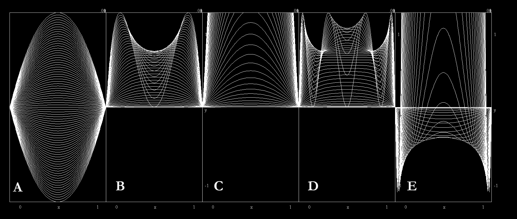
Figure 2: A, B and C, D and E illustrate, respectively, different positive (from 4 to 0) and negative (from 0 to -4)  values, step 0.1, for the equations (5), (6), (7).
The non ideal contribution to the free energy of a mixture
The molar free energy of mixing of a binary regular solution is given by:
 (8)
(8)
where  is the ideal mixing
  and
and  is the excess contribution
  respectively.
The non ideal contribution to the free energy, , is a symmetrical function of composition:
 (9)
(9)
where  is the A-B interchange energy of interaction parameter and
  and
and  are respectively the mixture end-members, so:
 (10)
(10)
Thus
 (11)
(11)
Or otherwise
 (12)
(12)
where 
Hildebrand (1929) introduced the term regular solution for some types of solution which follow equation (10) and in which the interact parameter  is independent from P and T.
Guggenheim (1937) more generally suggested that the molar excess Gibbs energy of a binary solution may be represented by the polynomial expression:
 (13)
(13)
When the A constants with odd subscripts, A1, A3 etc are zero the  becomes symmetrical with respect to composition, and are, thus, called symmetric solutions by Guggenheim (1967). The simplest functional form of no ideal solution is the one in which all but the first constant in equation (13) is zero. In this case
  is the equation (9). Guggenheim (1967) called this type of solution a simple mixture. So for excess free energy of mixing, the term regular solution and simple mixture coincide.
Treatments beyond three or four components are generally rare despite the presence of many minor compounds in phases of geologic interest. This is essentially because of problems connected with computational aspects ( id. es. Whol 1946, 1953; Kohler 1960; Hillert, 1980) but the effort of each model was condensed on the possibility to describe rather than to understand the intrinsic properties of excess energies, so parameter numbers utilized pose a greater problem.
Verhulst's approach to excess energy of a mixture
As above illustrated, in biology logistic maps describe the evolution of a population in a limited area. This formulation is conceptually analogous to description of excess Gibbs energy in a mixture. In the same way eq. (11) and eq.(5) suggest interpreting the two-component excess free energy of a mixture as a coupled logistic model (in a binary case as the dynamics of two isolated metaphorical symbiotic species). Mathematically, logistic map equations allows us to give an explicit parametric representation of the phenomenon rather than adopt an implicit formulation in more composite components solution ( as for example expressed by eq. 14). In this hypothesis each end-member can be treated with logistic-type dynamics. Excess energy is equal to the sum of partial energies of components present in the mixture as follows:
For a binary solution: (14)
(14)
Where  is eq.(10) and
  parameter is unique for each iteration number; this formulation allows us to adopt logistic maps as interpolation function. Generalizing expression. (14) to
  components, we have:
 (15)
(15) (16)
(16) which describes the overall dynamics can be named interaction evolution rate. It is remarkable that even a few iterations allow us to effectively describe the mixture, so in the present work the iteration has been expanded to the third order. The above expression, adopting this assumption, can be rewritten as:
 (17)
(17)
as will be explained in depth later.
Applications
From equation (9) adopting (17), Verhulst's approach can be summed up, operatively, as follows respectively for a binary (18), ternary (19) and quaternary (20) system:
 (18)
(18)
 (19)
(19) (20)
(20)where, as before described, (5), (6), (7) different iteration degrees are singularly
 (21)
(21)
To evaluate the significance of the logistic model, for comparison we have utilized experimental data utilized by Wilson (1964) and Kholer and Findenegg (1965) to validate their own models.
So for binary set illustrated in table 1 (Wilson, 1964):
Methanol-Benzene(MB)
While for ternary set exemplified in table2a (Wilson, 1964) and 2b (Kholer and Findenegg, 1965):
Methanol-CarbonTetrachloride-Benzene(MCB) Acetone-Methanol-Methilacetate (AMM)
Acetone-Methanol-Chloroform (AMC) Acetone-Methanol-Water (AMW)
nButane-Butene-Furfurole (NBF) Methane-Tetrachlore-Benzol (MTB)
Aniline-Cycloexane-Benzol (ACB) Ethanol-Dichloreethane-Benzol (EDB)
Heptane-Cyclohexane-Benzol (HCB) Tetrachlore-Cyclohexane-Benzol (TCB)
Futhermore, there are few references to studied quaternary excess solution systems and none for quintenary systems are actually available. For quaternary dataset we have considered the pyroxene MCCF (Mg2Si2O6-CaMgSi2O6-CaFeSi2O6-FeSi2O6) system described by Ottonello,1992 (table3).
As appears manifest in tables 1 and 2, below illustrated, the efficacy of the logistic map approach is not particularly convenient for binary and ternary systems because the coefficient number is greater compared to other models and the mean error is substantially the same. The situation changes radically from quaternary compositions ( e.g.. Wohl model needs 17 interaction parameters (12 binary, 4 ternary and 1 quaternary) while 12 are required by the logistic map model). Differences increase further with more complicated compositions. Table 4 summarizes adopted parameters calculated in tables 1 and 2.
Table 1: Excess enthalpy of mixing for vapour-liquid equilibrium data (Wilson, 1964) of the system Methanol-Benzene at 35°C, values calculated with present model and discrepancies between experimental and calculated data.
XMethanol Gexcess,cal/mole calculated delta delta Wilson
_____________________________________________________
0.0242 47.150 35.625 11.524 7.20
0.0254 40.670 37.288 3.381 -1.21
0.1302 173.40 157.681 15.718 5.73
0.3107 281.08 281.080 1.2E-5 1.59
0.4987 306.06 311.486 5.426 1.68
0.5191 304.24 309.096 4.856 1.17
0.6305 278.46 278.142 0.317 0.85
0.7965 192.65 184.120 8.529 0.76
0.9197 89.15 83.610 5.539 0.70
mean error 6.143 2.32
Table 2a: Comparison between experimental data from Wilson (1964) and present model (1). Table also details differences between experimental data of this model (2) and Wilson's results (3).
______________________________________________________________________
Methanol-Carbon Tetrachloride-Benzene
X1 X2 X3 deltaGsp deltaGcal (1) delta(2) delta(3)
_________________________________________________________________________
0.2075 0.19 0.6025 248.3 248.299 0.001 -0.5
0.211 0.3879 0.4011 257.6 273.450 15.850 -1.5
0.1987 0.5876 0.2137 253.6 253.600 9.37E-5 1.4
0.3781 0.3122 0.3097 320.5 320.500 5.52E-5 -0.9
0.5543 0.2078 0.2379 314.3 307.528 6.771 0.5
0.7599 0.1076 0.1325 225.2 225.200 0.001 1.6
mean error 3.770 1.06
Table 2b: Comparison between experimental data and Kohler's model (1960) from Kohler and Fingenegg (1965) and proposed model (2) calculations. the table also details the differences between experimental data and Kohler's model (3) and experimental data and Verlhust's model (4)
_________________________________________________________________________________
Acetone-Methanol-Methyacetate
X1 X2 X3 deltaGsp deltaGcal (1) deltaGcal(2) delta(3) delta(4)
_________________________________________________________________________________
0.066 0.872 0.062 57.800 61.500 76.110 -3.700 18.310
0.065 0.875 0.060 57.600 60.100 74.737 -2.500 17.137
0.577 0.342 0.081 90.000 95.500 90.000 -5.500 2.7E-5
0.883 0.067 0.050 26.500 24.100 26.500 2.400 0.001
0.421 0.457 0.122 118.200 108.800 115.878 9.400 2.321
0.434 0.442 0.124 112.900 108.800 113.547 4.100 0.557
0.539 0.273 0.188 94.000 96.100 83.281 -2.100 10.718
0.184 0.610 0.206 128.000 120.600 133.119 7.400 5.119
0.185 0.605 0.210 134.000 121.900 133.338 12.100 0.661
0.256 0.428 0.316 142.000 127.200 124.823 14.800 17.176
0.102 0.433 0.465 134.300 146.000 139.464 -11.700 5.164
0.110 0.430 0.460 137.400 144.000 138.431 -6.600 1.031
0.159 0.411 0.430 146.900 138.000 132.233 8.900 14.666
0.160 0.410 0.430 147.800 138.000 132.056 9.800 15.743
0.454 0.097 0.449 56.000 60.700 86.242 -4.700 30.242
0.472 0.063 0.465 49.900 47.300 85.659 2.600 35.759
0.232 0.215 0.553 104.800 103.900 104.799 0.900 0.001
0.101 0.235 0.664 110.700 113.000 106.980 -2.300 3.719
mean error 6.194 9.907
Acetone-Methanol-Chloroform
X1 X2 X3 deltaGsp deltaGcal (1) deltaGcal(2) delta(3) delta(4)
_________________________________________________________________________________
0.045 0.902 0.053 31.300 50.100 95.432 -18.800 64.132
0.483 0.483 0.035 107.600 87.000 82.729 20.600 24.870
0.453 0.500 0.047 81.600 83.600 92.554 -2.000 10.954
0.493 0.466 0.041 100.000 84.500 75.827 15.500 24.172
0.896 0.052 0.052 5.500 -3.500 -39.125 9.000 44.625
0.195 0.622 0.183 79.900 99.600 165.183 -19.700 85.282
0.200 0.600 0.200 82.500 84.500 162.564 -2.000 80.064
0.433 0.432 0.135 75.100 78.500 75.099 -3.400 0.001
0.600 0.200 0.200 3.300 20.200 -31.143 -16.900 34.443
0.574 0.207 0.219 8.300 21.900 -25.896 -13.600 34.196
0.024 0.500 0.476 173.200 186.300 171.544 -13.100 1.655
0.026 0.508 0.466 175.300 183.100 173.376 -7.800 1.923
0.026 0.487 0.487 168.000 183.100 167.997 -15.100 0.003
0.154 0.433 0.413 107.600 128.000 135.420 -20.400 27.820
0.333 0.333 0.333 52.600 71.000 63.559 -18.400 10.959
0.427 0.146 0.427 -39.600 -6.800 -14.336 -32.800 25.263
0.498 0.029 0.473 -113.900 -96.500 -43.459 -17.400 70.440
0.492 0.027 0.481 -121.200 -98.600 -42.403 -22.600 78.796
0.487 0.026 0.487 -148.400 -100.000 -41.502 -48.400 106.897
0.200 0.200 0.600 53.200 65.800 47.237 -12.600 5.962
0.190 0.196 0.614 60.900 66.900 47.617 -6.000 13.282
0.048 0.046 0.906 22.300 17.900 15.821 4.400 6.478
mean error 15.477 34.192
Acetone-Methanol-water
X1 X2 X3 deltaGsp deltaGcal (1) deltaGcal(2) delta(3) delta(4)
_________________________________________________________________________________
0.607 0.330 0.063 109.000 108.400 162.431 0.600 53.431
0.257 0.640 0.103 116.500 105.500 116.487 11.000 0.013
0.672 0.082 0.246 205.600 219.300 205.600 -13.700 2.26E-6
0.275 0.344 0.381 222.200 223.700 213.883 -1.500 8.316
0.075 0.470 0.455 162.300 158.400 203.582 3.900 41.282
0.361 0.127 0.512 267.100 294.000 266.793 -26.900 0.306
0.158 0.088 0.754 223.500 208.900 223.585 14.600 0.085
0.066 0.119 0.815 165.700 131.100 187.806 34.600 22.106
mean error 13.350 15.692
n-Butane-Butene-Furfurole
X1 X2 X3 deltaGsp deltaGcal (1) deltaGcal(2) delta(3) delta(4)
_________________________________________________________________________________
0.027 0.205 0.768 186.600 185.400 186.600 1.200 8.6E-7
0.038 0.187 0.776 185.500 183.700 186.226 1.800 0.726
0.045 0.216 0.739 198.300 196.400 194.110 1.900 4.189
0.099 0.133 0.768 199.500 194.300 198.754 5.200 0.745
0.166 0.036 0.798 200.500 199.000 202.232 1.500 1.732
0.069 0.094 0.837 162.200 159.000 165.540 3.200 3.340
0.147 0.030 0.823 186.200 185.100 186.193 1.100 0.001
0.021 0.112 0.868 130.600 130.100 140.317 0.500 9.717
0.113 0.024 0.863 158.100 156.200 155.090 1.900 3.009
mean error 2.033 2
Methanol-Tetrachlore-Benzol
X1 X2 X3 deltaGsp deltaGcal (1) deltaGcal(2) delta(3) delta(4)
_________________________________________________________________________________
0.843 0.081 0.075 168.800 172.800 179.133 -4.000 10.333
0.752 0.112 0.137 238.000 240.100 238.001 -2.100 0.001
0.195 0.592 0.213 253.000 241.600 253.000 11.400 0.001
0.556 0.213 0.231 324.600 317.100 289.441 7.500 35.158
0.359 0.323 0.318 324.600 307.300 280.496 17.300 44.103
0.198 0.396 0.406 252.300 234.500 263.538 17.800 11.238
0.198 0.396 0.406 251.100 234.500 263.538 16.600 12.438
0.188 0.196 0.616 235.300 222.800 232.298 12.500 0.001
mean error 11.150 14.159
Aniline-Cyclohexane-Benzol
X1 X2 X3 deltaGsp deltaGcal (1) deltaGcal(2) delta(3) delta(4)
_________________________________________________________________________________
0.148 0.442 0.410 155.500 153.600 155.500 1.900 1.89E-5
0.204 0.238 0.558 135.300 141.800 134.966 -6.500 0.333
0.273 0.245 0.482 183.400 168.700 160.485 14.700 22.914
0.300 0.375 0.325 198.300 175.400 178.298 22.900 20.002
0.411 0.224 0.365 229.500 191.700 197.366 37.800 32.133
0.509 0.136 0.355 216.000 170.200 215.165 45.800 0.834
0.557 0.206 0.237 233.900 201.800 212.352 32.100 21.547
0.656 0.139 0.205 187.400 170.900 208.082 16.500 20.682
mean error 22.275 14.805
Ethanol-Dichlorathane-Benzol
X1 X2 X3 deltaGsp deltaGcal (1) deltaGcal(2) delta(3) delta(4)
_________________________________________________________________________________
0.603 0.339 0.058 232.800 221.500 222.932 11.300 9.867
0.241 0.658 0.101 208.100 198.000 208.099 10.100 0.001
0.139 0.751 0.110 145.200 133.500 148.807 11.700 3.607
0.736 0.134 0.130 182.300 173.600 182.321 8.700 0.021
0.400 0.433 0.167 254.300 235.300 253.498 19.000 0.801
0.143 0.626 0.231 130.900 135.000 166.752 -4.100 35.852
0.478 0.261 0.261 263.800 241.100 262.666 22.700 1.133
0.600 0.059 0.341 248.700 237.100 261.544 11.600 12.844
0.430 0.169 0.401 263.500 249.900 282.572 13.600 19.072
0.301 0.347 0.352 234.700 222.100 229.506 12.600 5.193
0.209 0.401 0.390 195.300 184.300 189.018 11.000 6.281
0.282 0.106 0.612 239.900 231.400 239.910 8.500 0.010
0.121 0.268 0.611 134.900 130.200 149.751 4.700 14.851
0.123 0.123 0.754 138.300 136.000 136.520 2.300 1.779
mean error 10.850 7.951
Heptane-Cyclohexane-Benzol
X1 X2 X3 deltaGsp deltaGcal (1) deltaGcal(2) delta(3) delta(4)
_________________________________________________________________________________
0.044 0.139 0.817 136.200 134.100 151..969 2.100 15.769
0.060 0.188 0.752 166.600 168.500 180.154 -1.900 13.554
0.088 0.120 0.792 160.800 156.800 160.800 4.000 4.01E-6
0.099 0.058 0.843 130.300 132.900 136.831 -2.600 6.531
0.120 0.070 0.810 155.100 153.700 153.465 1.400 1.634
0.166 0.195 0.639 204.600 221.300 206.878 -16.700 2.278
0.155 0.250 0.595 216.100 229.200 215.246 -13.100 0.853
0.158 0.380 0.462 226.800 235.400 223.598 -8.600 3.201
0.160 0.505 0.335 195.500 205.500 206.779 -10.000 11.279
0.119 0.684 0.197 147.200 131.900 147.412 15.300 0.212
0.304 0.195 0.501 226.100 240.000 221.437 -13.900 4.662
0.280 0.259 0.461 220.600 240.700 220.471 -20.100 0.128
0.243 0.342 0.415 228.700 236.800 218.537 -8.100 10.162
0.286 0.387 0.327 210.300 217.700 208.742 -7.400 1.557
0.311 0.418 0.271 176.100 197.900 200.742 -21.800 24.754
0.422 0.280 0.298 195.700 206.700 199.639 -11.000 3.939
0.447 0.237 0.316 197.900 209.100 199.791 -11.200 1.891
0.577 0.191 0.232 170.900 170.200 168.175 0.700 2.724
0.625 0.169 0.206 154.200 155.100 154.307 -0.900 0.106
mean error 8.989 5.539
Tetrachlore-Cyclohexane-Benzol
X1 X2 X3 deltaGsp deltaGcal (1) deltaGcal(2) delta (3) delta(4)
_________________________________________________________________________________
0.213 0.574 0.213 109.700 110.200 111.684 -0.500 1.984
0.233 0.534 0.233 115.300 113.500 115.300 1.800 4.07E-5
0.280 0.440 0.280 120.500 115.000 119.272 5.500 1.227
0.306 0.388 0.306 118.200 113.600 118.688 4.600 0.488
0.325 0.350 0.325 117.200 111.400 117.168 5.800 0.031
mean error 3.640 0.746
Table 3: Energy parameters of C2/c pyroxene quadrilateral calculated on 55 distinct compositions by Ottonello (1986) evaluated with Verlhust's approach and discrepancies between data.
_________________________________________________________________________________
X1 X2 X3 X4 deltaGmodel deltaGcalculated delta
_________________________________________________________________________________
0.0000 0.5000 0.5000 0.0000 0.001 7.998 7.997
0.0500 0.5000 0.4500 0.0000 1.669 6.804 5.135
0.1000 0.5000 0.4000 0.0000 2.608 5.782 3.174
0.1500 0.5000 0.3500 0.0000 3.622 4.948 1.326
0.2000 0.5000 0.3000 0.0000 4.323 4.315 0.007
0.2500 0.5000 0.2500 0.0000 4.266 3.898 0.367
0.3000 0.5000 0.2000 0.0000 3.713 3.712 0.001
0.3500 0.5000 0.1500 0.0000 3.572 3.772 0.200
0.4000 0.5000 0.1000 0.0000 2.320 4.091 1.771
0.4500 0.5000 0.0500 0.0000 1.196 4.685 3.489
0.5000 0.5000 0.0000 0.0000 0.001 5.568 5.567
0.0000 0.4000 0.5000 0.1000 4.059 8.490 4.431
0.0830 0.4000 0.4170 0.1000 6.614 6.601 0.012
0.1670 0.4000 0.3330 0.1000 7.114 5.201 1.912
0.2500 0.4000 0.2500 0.1000 8.013 4.390 3.622
0.3330 0.4000 0.1670 0.1000 7.240 4.215 3.024
0.4170 0.4000 0.0830 0.1000 4.807 4.753 0.053
0.5000 0.4000 0.0000 0.1000 2.765 6.060 3.295
0.0000 0.3000 0.5000 0.2000 6.556 8.182 1.626
0.0715 0.3000 0.4285 0.2000 8.291 6.527 1.763
0.1425 0.3000 0.3575 0.2000 9.653 5.244 4.408
0.2140 0.3000 0.2860 0.2000 10.279 4.360 5.918
0.2860 0.3000 0.2140 0.2000 9.242 3.924 5.317
0.3575 0.3000 0.1425 0.2000 7.729 3.986 3.742
0.4285 0.3000 0.0715 0.2000 6.325 4.579 1.745
0.5000 0.3000 0.0000 0.2000 4.174 5.752 1.578
0.0000 0.2000 0.5000 0.3000 6.922 7.254 0.332
0.0625 0.2000 0.4375 0.3000 8.275 5.788 2.486
0.1250 0.2000 0.3750 0.3000 8.963 4.597 4.365
0.1875 0.2000 0.3125 0.3000 9.437 3.709 5.727
0.2500 0.2000 0.2500 0.3000 9.009 3.154 5.854
0.3125 0.2000 0.1875 0.3000 9.050 3.766 6.090
0.3750 0.2000 0.1250 0.3000 7.617 4.824 4.462
0.4375 0.2000 0.0625 0.3000 6.530 3.766 2.763
0.5000 0.2000 0.0000 0.3000 4.278 4.824 0.546
0.0000 0.1000 0.5000 0.4000 4.920 5.886 0.966
0.0555 0.1000 0.4445 0.4000 5.500 4.571 0.928
0.1110 0.1000 0.3890 0.4000 5.968 3.457 2.497
0.1670 0.1000 0.3330 0.4000 6.102 2.597 3.504
0.2225 0.1000 0.2775 0.4000 5.686 1.987 3.698
0.2775 0.1000 0.2225 0.4000 6.163 1.654 4.508
0.3330 0.1000 0.1670 0.4000 5.880 1.611 4.268
0.3890 0.1000 0.1110 0.4000 5.267 1.885 3.381
0.4445 0.1000 0.0555 0.4000 4.438 2.493 1.944
0.5000 0.1000 0.0000 0.4000 3.203 3.456 0.253
0.0000 0.0000 0.5000 0.5000 0.001 4.257 4.256
0.0500 0.0000 0.4500 0.5000 -0.007 3.063 3.070
0.1000 0.0000 0.4000 0.5000 0.334 2.041 1.707
0.2000 0.0000 0.3000 0.5000 0.135 0.573 0.438
0.2500 0.0000 0.2500 0.5000 0.077 0.156 0.079
0.3000 0.0000 0.2000 0.5000 -0.029 -0.029 5.4-E-6
0.3500 0.0000 0.1500 0.5000 -0.188 0.030 0.218
0.4000 0.0000 0.1000 0.5000 -0.069 0.349 0.418
0.4500 0.0000 0.0500 0.5000 -0.377 0.943 1.320
0.5000 0.0000 0.0000 0.5000 0.001 1.827 1.826
_________________________________________________________________________________
mean error 2.607
Table 4: Parameters of Verlhust's approach for binary, ternary and quaternary systems.
MB MCB AMM AMC AMW BBF MTB ACB EDB HCB TCB MCCF
 1065.545 2217.894 231.752 -930.942 1027.970 607.004 1486.731 1182.059 2374.026 801.718 468.956 82.606
 9.076 22.279 10.508 4.594 13.761 -19.456 8.090 7.789 25.070 14.996 13.801 -3.04E-6
 3.459 4.935 2.962 3.122 5.863 0.988 0.318 1.251 1.051 6.225 1.026 -0.040
 1424.870 1123.512 758.979 1209.642 303.189 -396.430 1176.158 497.238 82.387 791.600 632.982 -38.057
 8.336 13.022 0.010 -0.039 -5.253 20.542 -2.619 -11.467 -16.035 9.388 13.251 1.78E-5
 4.145 1.716 -2.265 -2.105 5.505 1.490 1.059 0.989 0.970 80.25 1.079 0.090
 - 957.835 487.593 168.983 1524.212 1372.701 1068.244 731.026 791.064 1208.905 468.956 102.047
 - 0.000 2.998 4.139 17.194 -7.186 2.072 16.831 11.350 13.098 13.801 -4.33E-7
 - 0.000 0.007 3.040 -4.514 -1.113 1.137 1.184 1.102 -1.942 1.026 0
 - - - - - - - - - - - -67.989
 - - - - - - - - - - - -1.46E-6
 - - - - - - - - - - - -0.095
Discussion and conclusions
There are some notable aspects to Verhulst's approach to excess energy of a mixture:
1) Physical: a logistic map describes the evolution of a population (Odum, 1983) . In the broad sense the population can be assumed as the amount of an end-member in a mixture.
2) Chemical: a logistic equation has already been used in chemistry to describe chemical evolution of a system (Latham, 1964; Northrop et al.,1948; Steven, 1965)
3) Mathematical: a logistic map appears to imitate the behavior of excess free energy in mixture processes as the tendency for like atoms to cluster.
The logistic map, used in population dynamics, allows us to indicate the growth rate of a population with limited resources. A mixture, in the same manner, is conditioned by environment. It is important to recognize that a twice iterated logistic map is equal to a once-iterated fourth degree polynomial, mimicking the atom's tendency to cluster.
Mathematically, a logistic map as the recursive function of non-ideal contribution to free energy (eq. 11), is intrinsically consistent both with theory, and with the natural recursivity of crystallographic structure because the purpose of interaction between end-member, analogously to a biotic system, is optimization of the energy asset efficiency. Experimental data validates the acceptability of the model.
References
Cheng, W. and Ganguly, J. (1994): Some aspects of multicomponent excess free energy models with subregular binaries. Geochim. Cosmochim. Acta, 58:3763-3767.
Guggenheim E.A. (1937) Theoretical basis of Raoult'law. Trans. Faraday Soc., 33, 151-159
Guggenheim E.A. (1967) Thermodynamics. Amsterdam, North. Holland Publ. Co.
Hildebrand J.H. (1929) Solubility, XII, Regular solutions. J.Am. Chem.Soc.,51, 66-80
Hillert M. (1980) Empirical methods of predicting and representing thermodynamic properties of ternary solution phases. Calphad 4, 1-12
Kohler F. & Findenegg G.H. (1965) Zur Berechnung der Thermodynamischen Daten eines ternaren System aus den zugehorigen binaren systemen. Monatschr Chem., 96, 1229-1251
Kohler F. (1960) Zur Berechnung der Thermodynamischen Daten eines ternaren System aus den zugehorigen binaren systemen. Monatschr Chem., 91, 738-740
Latham J. L. (1964) Elementary reaction kinetics. London Butterworths.
Lotka A. J. (1956) Elements of physical biology. Baltimore, William & Wilkins 460 pp. (reprinted as Elements of mathematical biology New York, Dover 1956.)
May R.M. (1976) Simple mathematical models with very complicated dynamics, Nature 261, 459-467.
Northrop J.H., Kenitz M. and Heniot R.M. (1948) Crystalline enzymes 2nd ed. New York Cambridge University Press
Odum E. P. (1983) Basic Ecology CBS College Publishing 544 pp.
Ottonello G. (1992) Interactions and mixing properties in the (C2/c) clinopyroxene quadrilateral Contrib. Mineral. Petrol., 111, 53-60
Steven B. (1965) Chemical kinetics for general students of chemistry. London Chapman & Hall
Tsallis (1995) Non-extensive themostatistics brief review and comments. Physica A 221, 277-290
Tsallis (1999) Nonextensive statistics: theoretical, experimental and computational evidences and connections. Brasilian Journal of Physics 29, 1-35
Verhulst P.F. "Deuxième mémoire sur la loi d'accroissement de la population." Mém. de l'Academie Royale des Sci., des Lettres et des Beaux-Arts de Belgique 20, 1-32, 1847.
Verhulst P.F. "Recherches mathématiques sur la loi d'accroissement de la population." Nouv. mém. de l'Academie Royale des Sci. et Belles-Lettres de Bruxelles 18, 1-41, 1845.
Wilson G.M. (1964) Vapour-liquid equilibrium XI. A new expression for the excess free energy of mixing. J. Am. Chem. Soc., 86, 127130
Wohl K. (1946) Thermodynamic evaluation of binary and ternary liquid systems. Trans Am. Inst. Chem Eng., 42, 215-249